Time-domain Analysis

The problem and the solution

A fundamental aspect of loudspeaker modeling is the ability to calculate the time-domain response of a driver in free air, or in a specified enclosure, given prior calculation of the frequency response. Whereas the low-frequency electroacoustic theory of Benson, Thiele and Small may be used to compute the steady-state pressure (SPL), velocity and excursion of a loudspeaker as a function of frequency, it remains to compute the time-domain impulse and step responses by inverse Laplace transform. This is done analytically by Benson [Ben93] for simple closed boxes by decomposing the \(s\)-domain response function into a sum of poles such that the Laplace transform can be inverted using exponential and related functions. For more complicated polynomial filters, numerical methods based on computing eigenvalues of the companion matrix are often used. This approach does not generalize to non-polynomial response functions which inevitably require a numerical treatment, most often by discrete Fourier inversion methods.

In these notes we describe a numerical approach to invert Laplace transforms required for computation of the time-domain response of loudspeakers. The method is an adaptation of the method of Weideman [WT07], with suitable modifications to accomodate the analytic structure found in typical audio applications. In comparison to Fourier method, however, the Weideman method is significantly more efficient and accurate, yet it is straightforward to implement without the need for third-party mathematical libraries. Thus it can be implemented in existing box-modeling software with little effort.

Response function representation

Consider the driven linear system

(27)\[{\cal D} \, x(t) = f(t) \; ,\]

where \(x\) is a generalized displacement, \(f\) is a generalized force, and \({\cal D}\) is a linear operator. We remark that \({\cal D}\) can contain integrals, derivatives or fractional derivatives. Taking the Laplace transform of Eq. (27) and solving for \(X(s)\) yields the response function form of the linear system:

\[X(s) = R(s) F(s) \; .\]

Here, \(X(s)\) and \(F(s)\) are the Laplace transforms of \(x(t)\) and \(f(t)\),

\[\begin{split}\begin{eqnarray} X(s) & = & {\cal L}[x] \doteq \int_0^\infty dt \, e^{-st} x(t) \; , \\ F(s) & = & {\cal L}[f] \doteq \int_0^\infty dt \, e^{-st} f(t) \; . \end{eqnarray}\end{split}\]

and \(R(s)\) is the response function. One can solve for \(x(t)\) by inverting the Laplace transform

\[x(t) = {\cal L}^{-1} \left[ R(s) F(s) \right] \; ,\]

where the inverse is defined in terms of the Bromwich integral

(28)\[x(t) = {\cal L}^{-1} \left[ X \right] \doteq \frac{1}{2 \pi i} \int_{\sigma-i\infty}^{\sigma+i\infty} ds \, e^{st} X(s) \; .\]

Here, \(\sigma\) is chosen so that the contour lies to the right of all singularities of the integrand, as illustrated in Fig. 20. So long as the contour remains to the right of these singularities, the Cauchy integral theorem [GK06] guarantees that the value of the integral is independent of the path of integration.

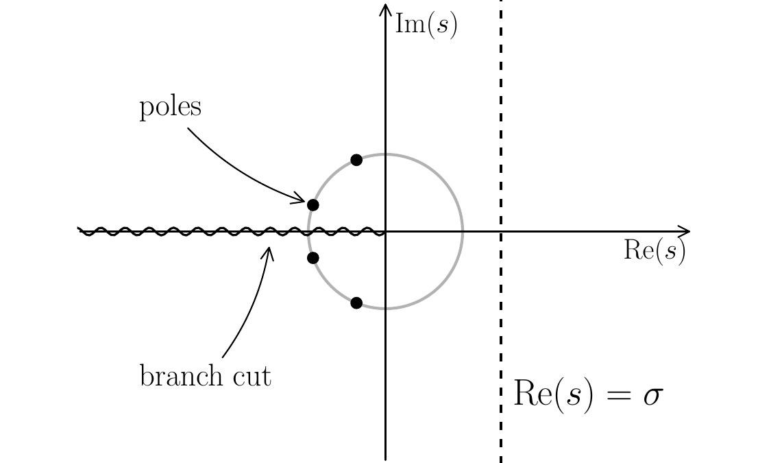
Fig. 20 Complex plane illustrating Bromwich inversion contour (dashed line) for a hypothetical case. The contour must lie to the right of all poles and branch cuts. Also shown is the unit circle, poles typical of a 4^th-order Butterworth filter, and a branch cut (wavy curve) at \(s=0\).

Impulse response

The impulse response is generated using the Dirac delta function \(\delta(t)\) as the driving force:

\[f(t) = \delta(t) \Longleftrightarrow F(s) = 1 \; .\]

The required inverse transform is thus

\[\xim(t) = {\cal L}^{-1} \left[R(s)\right] \; .\]

In the solution of inhomogeneous differential equations, when \(\cal{D}\) is a linear differential operator, the impulse response \(\xim\) is equivalently called the Green’s function for (27).

Step response

The step response is generated using the Heaviside step function \(H(t)\) as the driving force:

\[f(t) = H(t) \Longleftrightarrow F(s) = 1/s\]

The required inverse transform is thus

\[\xs(t) = {\cal L}^{-1} \left[\frac{R(s)}{s}\right]\]

The step and delta functions are related according to

\[\frac{dH}{dt} \doteq \dot{H} = \delta(t) \; ,\]

where this formula is rigorously justified in terms of generalized functions [Zem65]. Note that, in this paper, a dot denotes a time derivative.

General system response

Using the convolution property of the inverse transform, it is easy to show that

\[\begin{split}\begin{eqnarray} x(t) &=& \int_0^t d\tp \, \xim(\tp) f(t-\tp) \; , \\ &=& \int_0^t d\tp \, \xs(\tp) \dot{f}(t-\tp) \; . \end{eqnarray}\end{split}\]

Evidently, one can also compute the step response by integration of the impulse response,

\[\xs(t) = \int_0^t d\tp \, \xim(\tp) \; .\]

A simple example outlining the calculation of impulse and step responses for a simple linear oscillator is given in the Appendix. In the following sections we will focus on the step response, \(\xs\), because it avoids the singularity present in the impulse response. The step response is typically computed in box modeling programs.

Application to transducer response

In the present paper, we choose to formulate the inverse problem using a dimensionless time \(t = \ws \tau\), where \(\tau\) is the physical time, and \(\ws = 2 \pi \fs\) is the resonant frequency of the loudspeaker driver. To illustrate the inversion process for a simple case, we consider the steady-state pressure response for an undamped, closed box [Ben93]. In this case, the response function takes the form of a 2^nd-order high-pass filter

(29)\[R(s) = \frac{s^2}{\displaystyle s^2 + \frac{s}{\qts} + 1 + \alpha} \; ,\]

where \(\alpha \doteq \cms/\cmb\) is the compliance ratio and \(\qts\) is the driver total \(Q\). In these expressions, \(\cms\) is the mechanical compliance of the driver suspension, and \(\cmb\) is the equivalent mechanical compliance of the interior of the closed box. Further, \(1/\qts = 1/\qes + 1/\qms\), where \(\qes\) and \(\qms\) are the electrical and mechanical \(Q\) factors of the driver.

For the special choice of \(\alpha=0\) (i.e., the infinite baffle limit \(\cmb \rightarrow \infty\)) and \(\qts = 0.5\), we can write the inversion integral for the step response as

(30)\[\xs(t) = \frac{1}{2 \pi i} \int_{\sigma-i\infty}^{\sigma+i\infty} ds \, e^{st} \, \frac{s}{s^2 + 2s + 1} \; .\]

The integrand contains a pole of order 2 at \(s=-1\), in which case we can close the contour to the left and use the residue theorem to give

(31)\[\xs(t) = \frac{\partial}{\partial s}\left. \left(s e^{st}\right) \right|_{s = -1} = e^{-t} (1-t) \; .\]

In the more realistic case of vented and damped enclosures, the same method based on analytic contour integration will work in principle, although locating the poles and computing residues may become tedious and complicated. In practical cases, the residue calculation is done numerically by computing eigenvalues of the companion matrix [EM95]. Importantly, the residue-based methods described above are applicable only to rational functions, and fail in the general case for which the driver circuit model contains semi-inductance [TF11] or viscoelastic creep [KJ93, Nov16, TF13, TTAF10]. In this case the frequency-domain response function will contain elements described by functions with branch points – for example, \(\sqrt{s}\) or \(\ln(s)\). One must then return to the Bromwich integral in Eq. (28) and perform the contour integration numerically.

The problem of numerical inversion of the Laplace transform has been an active area of research since the 1960s [BKK66], with an important method developed by Talbot in 1979 [Tal79]. There is no single best method; rather, the most suitable method will in general depend on the nature of the problem. To illustrate the convergence issues associated with inversion of the transform, consider again the example of Eq. (30). As a straightforward attempt to evaluate the Bromwich integral directly, one can put the integration contour on the imaginary axis \(s=iy\). In this case the Bromwich integral, Eq. (30), reduces to the inverse Fourier transform

(32)\[\xs(t) = \frac{1}{2\pi} \int_{-\infty}^\infty dy \, e^{i y t} \, \frac{iy}{(iy)^2 + 2iy + 1} \; .\]

The conversion of the Bromwich integral to a Fourier integral is always possible when the singularities of the transfer function lie in the left half-plane (i.e., when the linear system is stable). This integral can be performed analytically to yield

(33)\[\begin{split}\begin{eqnarray} \xs(t) & = &~ \frac{1}{\pi} \int_0^\infty dy \, \frac{2y^2 \cos(yt) + (y^3-y) \sin(yt)}{(1+y^2)^2} \; , \\ & = &~ e^{-t} (1-t) \; . \end{eqnarray}\end{split}\]

As required, the analytic solution in Eq. (33), obtained by direct integration of the infinite (Fourier) integral, is the same as that obtained in Eq. (31) by contour integration. However, consideration of the Fourier integral above reveals a serious deficiency; namely, that the integral decays very slowly at large values of \(y\):

\[\frac{2y^2 \cos(yt) + (y^3-y) \sin(yt)}{(1+y^2)^2} \sim \frac{\sin(yt)}{y} \; \text{as}\; y \rightarrow \infty \; .\]

Thus, at small times \(t \ll 1\), extremely large values of \(y\) (i.e., very high frequencies in the Fourier sense) must be retained to accurately evaluate the integral. This is in contrast to the previous contour integration, which can determine the integral exactly via any closed contour surrounding the pole at \(s = iy = -1\). The implication is that a numerical method based on integration along a vertical contour will be fundamentally inefficient, quite independent of the numerical quadrature method. Let us take this illustration further by explicitly constructing a numerical inversion, via inverse discrete Fourier transform (iDFT), and rewrite the integral as

(34)\[\xs(t) = \int_{-\wmax}^{\wmax} dy \, e^{iyt} \frac{R(iy)}{iy} + E(\wmax) \; .\]

Above, \(E(\wmax)\) is the error resulting from truncation of the limits of integration, and, as before, \(R(s) = s^2/(s^2+2s+1)\). If we let \(t_n = n \Delta t\) and \(y_k = k \Delta y\) then

(35)\[x_n = \sum_{k=-N/2}^{N/2-1} e^{2\pi i kn/N} \, G_k \; , \quad n = 0, \ldots, N-1 \; ,\]

where \(x_n\) is an approximation to \(\xs(t_n)\), \(G_k = R(ik\Delta y)/(ik)\), \(\wmax = N \Delta y/2\), and \(\Delta y \Delta t = 2\pi/ N\). Eq. (35) thus expresses \(x_n\) as the iDFT of \(G_k\). In the limit \(N \rightarrow \infty\), \(x_n\) will exactly recover the finite integral in Eq. (34), but will always differ from \(\xs(t_n)\) by the truncation error \(E(\wmax)\). To illustrate the poor accuracy obtained in a typical case, consider a transducer with \(\fs = 100\) Hz and choose \(f_\mathrm{max} = 32\) kHz and \(n=8000\). Then

\[|\xs(t_n) - x_n| \sim E(\wmax) \sim 1.5 \times 10^{-3} \; ,\]

when \(t_n \sim 0.1\). Considering the very high resolution, this is a surprisingly large truncation error. The error is not a consequence of any particular deficiency of the iDFT itself, but rather of the vertical Fourier contour. This issue is well-recognized in the literature and numerous methods to overcome the poor convergence have been developed.

Weideman method

Instead of the vertical contour, we will use an approach based on deforming the contour into the left half-plane. Although the basic approach is due to Talbot [Tal79], we use the more recent optimal method due to Weideman [WT07], with modifications to suit the problem of loudspeaker response. It should be emphasized that application of the method requires the response function to be known as an analytic function of the complex variable \(s\).

Weideman treats both a parabolic and hyperbolic contour, but we consider only the parabolic one:

(36)\[s(u) = \mu \left( i u + 1 \right)^2 \, , \quad - \infty < u < \infty \; .\]

The integration rule is trapezoidal

(37)\[\xs(t) = \frac{\Delta}{2\pi i} \sum_{k=-N}^N e^{s_k t} \frac{R(s_k)}{s_k} s^\prime(u_k) \; ,\]

where \(s_k \doteq s(u_k)\), \(s^\prime = ds/du = 2\mu(i-u)\) and \(u_k = k \Delta\). Although Eq. (37) provides a discrete approximation to the integral for any values of \(\Delta\) and \(\mu\), Weideman shows that the optimal parameters for the parabolic contour are

(38)\[\Delta_\mathrm{opt} = \frac{3}{N} \quad \text{and} \quad \mu_\mathrm{opt} = \frac{\pi}{12} \frac{N}{t} \; .\]

So long as the contour is acceptable (not passing through singularities during deformation into the parabola), the method is remarkably accurate. We remark that the algorithm can be applied for any value of \(t > 0\), and the optimal parameters must be recomputed for every value of \(t\) according to Eq. (38). In Ref. [WT07], the emphasis is on solving problems for which singularities lie on the negative real axis, in which case there are no restrictions on the smallness of \(\mu\). For \(t\) sufficiently large, however, the magnitude of \(\mu_\mathrm{opt}\) will shrink so much that a pole is crossed. Since we expect poles approximately in the range \(|s| \sim 1\) (for example, a Butterworth filter has all poles on the left half of the unit circle), we must ensure that \(2 \mu > y_\mathrm{max}\), where \(y_\mathrm{max}\) is the maximum height of a pole, and \(2 \mu\) is the point at which upper-half of the parabola intersects the imaginary axis. To see this, note from Eq. (36) that \(s(1) = \mu (1+i)^2 = 2i\mu\).

Application to box response

To modify the Weideman algorithm to prevent pole crossing, it is instructive to consider in detail the behaviour of the response function for an undamped, vented box. This is written as

\[R(s) = \frac{s^4}{\displaystyle \left(s^2+h^2\right) \left( 1 + \frac{s}{\qts} + s^2\right) + \alpha s^2} \; .\]

The new parameter \(h = \wpb / \ws\), where \(\wpb\) is resonant frequency of the vented enclosure, transforms the response into a 4^th-order filter with four poles in the left half-plane. Small [Sma73a] refers to \(h\) as the system tuning ratio. Typical vented alignments choose \(h \sim 1\). The pole locations for this response function can be computed analytically in some special cases – most notably when the denominator coincides with the 4^th-order Butterworth polynomial:

(39)\[\begin{split}\begin{eqnarray} h^2 & = & 1 , \; \alpha = \sqrt{2} \\ 1/\qts & = & 2\cos(\pi/8)+2\cos(3\pi/8) \doteq 1/Q_4 \; . \end{eqnarray}\end{split}\]

Note that \(Q_4 \simeq 0.382683\). Then the poles occur on the unit circle at \(s_k = \exp(i\theta_k)\), where

\[\theta_k = \left\{ \frac{5\pi}{8} , \frac{7\pi}{8} , \frac{9\pi}{8} , \frac{11\pi}{8}\right\} \; .\]

In the general case, the poles can be computed using a numerical root-finding method. In Fig. 21 we show the root locus for different parameter variations away from the Butterworth case.

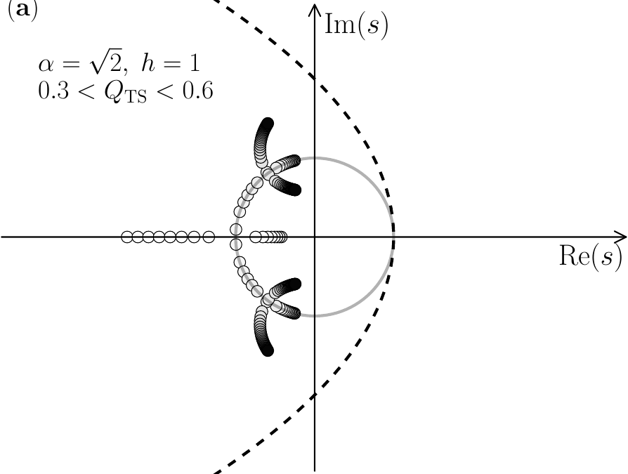
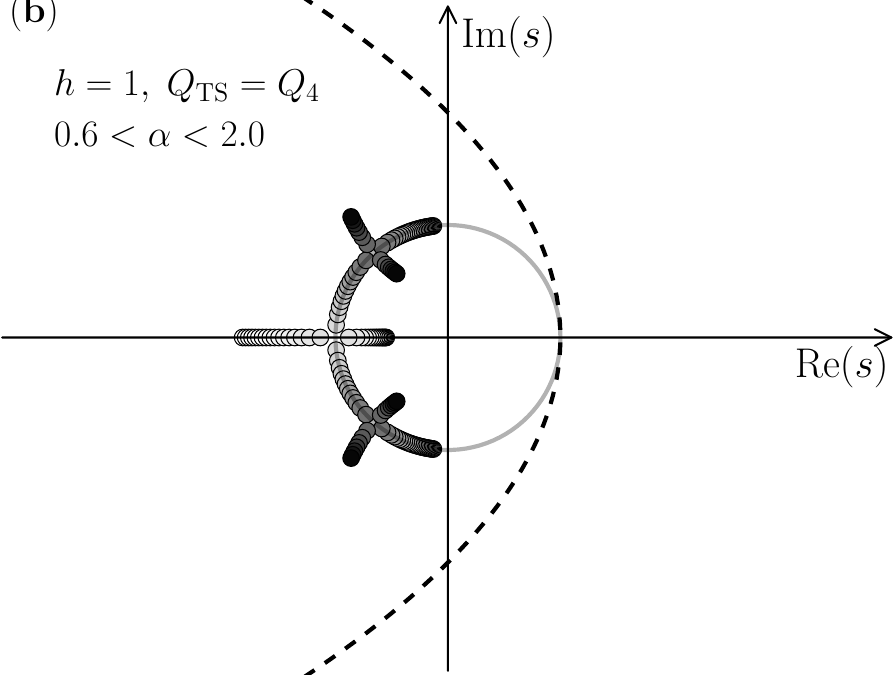
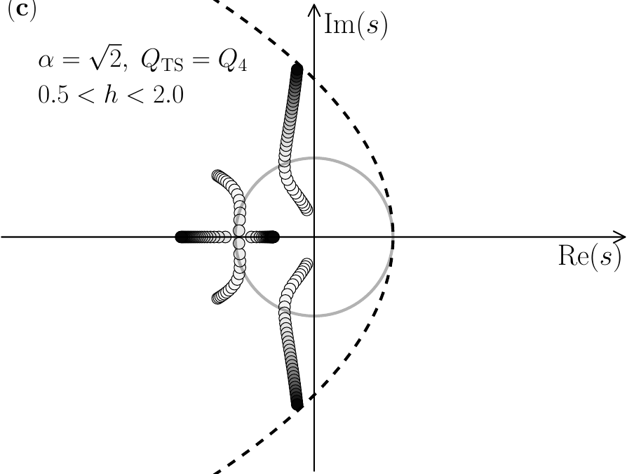
Fig. 21 Complex plane illustrating parabolic Weideman inversion contour for \(\mu=1\) and poles of the response function. Baseline parameter values are those for the Butterworth filter, as defined in Eqs. (39). Starting from the baseline values, we scan \(\qts\) in (a), \(\alpha\) in (b) and \(h\) in (c). Plot (c) shows that large values of \(h\) can give rise to a pole crossing, which must be avoided. Darker circles indicate larger values of the scanned parameter.

The root loci illustrate that, for a Butterworth filter, \(\mu > 1\) would be more than adequate to ensure that the parabolic contour always passes over the poles. However, in the limit of large tuning ratio, \(h \gg 1\), which corresponds to port tuning much higher than the driver resonant frequency, the two poles associated with the port resonance can be shown to occur at \(s \sim \pm i h -\alpha/(2h)\). This behaviour is illustrated in Fig. 21.c. Thus we would want to ensure that \(\mu > \max\left(1,h\right)\). Bearing these observations in mind, we can specify the required modifications to Weideman’s algorithm as follows: choose a value of \(N_0\) to give desired integration accuracy at short time. Using this value of \(N_0\), define the critical parameters

(40)\[\mu_c \doteq \max\left\{1,h\right\} \quad \text{and} \quad t_c \doteq \frac{\pi N_0}{12 \mu_c} \; .\]

If \(t < t_c\), set

(41)\[\mu = \frac{\pi N_0}{12 \, t} \;, \quad N = N_0 \; , \quad \Delta = \frac{3}{N}\]

Otherwise, for \(t \geq t_c\), choose

(42)\[\mu = \mu_c \; , \quad N = \left\lceil N_0 \, \frac{t}{t_c} \, \right\rceil \; , \quad \Delta = \frac{3}{N} \; ,\]

where \(\lceil \cdot \rceil\) is the ceiling function (i.e., the smallest integer greater than or equal to the argument). In other words, when \(t < t_c\), we decrease \(\mu\) at fixed \(N\) to stay on the optimal contour. When \(t > t_c\), we must increase \(N\) to stay on the optimal contour for fixed \(\mu_c\). In practice, the method is conservative insofar as \(N\) increases more rapidly than necessary to maintain accuracy. For more complicated response functions, some method to determine the maximum height of the pole should be used, and that value should replace \(h\) in the previous formulae. Since the minimum height of the parabolic contour in the left half-plane is \(y = 2 \mu\), the method above is conservative in that it ensures the contour is at least double the height of the highest pole. To justify this choice, refer again to Fig. 21 c. The plot shows that not only will the choice \(\mu=1\) fail when \(h > 2\), but that as the pole nears the contour, the integrand will vary rapidly, giving a large error in the trapezoidal integration scheme. Thus, the choice \(\mu_c \doteq \max\left(1,h\right)\) will ensure the contour is well-above the highest pole.

Result with viscoelastic suspension

To test the accuracy of the method for a more realistic case, we consider the previous vented box example but including the effects of viscoelastic compliance (suspension creep). For the compliance function we choose the so-called three-parameter creep (3PC) model of Ritter and Agerkvist [RA10].

(43)\[\cms \longrightarrow \clog \left[ 1-\beta \ln \left( \frac{s}{s+s_0} \right) \right] \; .\]

The 3PC model includes both logarithmic creep and frequency-dependent damping. It is a generalization of the earlier LOG model of suspension creep [KJ93], and introduces a parameter \(s_0\) to ensure that the frequency-dependent compliance \(\cms(s)\) is nonnegative at high frequency. The form of the compliance in Eq. (43) is equivalent to the original form given in Ref. [RA10], but written more compactly. Some aspects of the algebra required to establish the equivalence is given in the Appendix. We further remark that in Eq. (43), \(\beta\) is the parameter of viscoelasticity (the creep parameter), which in the work by Ritter and Agerkvist (and the original work by Knudsen and Jensen) was represented by \(\lambda\). The conversion between the representations is clarified in Appendix A.4 of Ref. [CF17].

Proceeding, the vented box response function can be modified to include the effects of viscoelasticity by writing

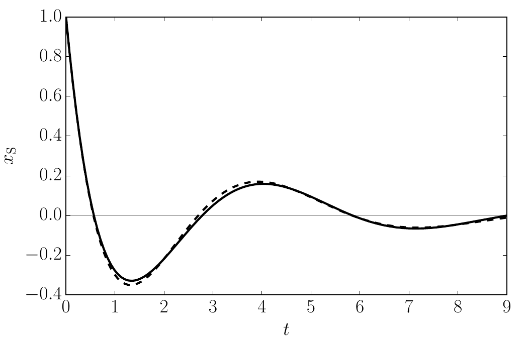
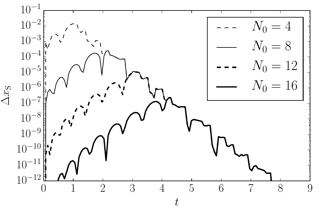
Fig. 22 Left plot shows time-domain step response \(\xs(t)\) corresponding to \(R(s)\) given in Eq. (44) with \(h\), \(\qts\) and \(\alpha\) corresponding to the Butterworth values. Time dependence is shown with creep (solid curve, \(\beta=0.5\)) and without creep (dotted curve, \(\beta=0\). Right plot shows absolute error, \(\Delta x_\mathrm{S} = | x_\mathrm{S}^{(N_0)}- x_\mathrm{S}^{(32)}|\), in inverse calculation for undamped vented box response function \(R(z)\). Here, \(x_\mathrm{S}^{(N_0)}\) refers to a numerical calculation with the given starting value \(N_0\).

(44)\[R(s) = \frac{s^4}{\displaystyle \left(s^2+h^2\right) \left( \frac{1}{c(s)} + \frac{s}{\qts} + s^2\right) + \alpha s^2} \; ,\]

where \(c(s)\) is an analytic function

\[c(s) \doteq 1-\beta \ln \frac{s}{s+2} \; ,\]

that multiplies the static suspension compliance, \(\clog\). In this example, we have chosen \(s_0=2\), corresponding to a transition frequency that is double the resonant frequency, but in practical cases other values may apply. Note that when replacing the static compliance with the 3PC model, the meaning of \(\rms\) will change in response to the frequency-dependent damping effect (originating from the imaginary part of the logarithm). We emphasize that due to the branch cut \(s \in [-2,0]\), the inverse transform of \(R(s)/s\) cannot be computed by traditional transform tables or a straightforward integration. Fig. 22 shows the time-domain step response as computed using the method of the present paper. The solid and dashed curves, respectively, show the response with and without the creep function. We can also give an indication of the resolution required to give acceptable results. Also in Fig. 22 we plot the absolute inversion error as a function of the initial number of nodes, \(N_0\). We remark that eventually all curves overlap at sufficiently large \(t\) for which \(\mu = 1\). These results show that the present method can compute the inverse efficiently to nearly machine precision. In fact, in generating Fig. 22, it was sufficient to use \(N_0 \leq 32\). This is surprising given the apparent computational complexity of the integral in Eq. (33).

Although the Fourier approach of Eq. (35) can be modified to give some accuracy improvement, it is manifestly less computationally efficient than the more elegant contour method. The latter with \(N = 2 N_0 + 1 = 17\) gives better accuracy than the Fourier method with \(N = 8000\), and with \(N = 65\) points, the modified Weideman contour method returns an answer correct to nearly the full machine precision!

Nonlinear driver simulation

To illustrate how the present inversion method can be applied to time-domain simulation of (nonlinear) driven loudspeaker response, consider the time-domain differential equations that describe the driver displacement \(x(\tau)\) [Kai87]:

(45)\[\begin{split}\begin{eqnarray} V(\tau) &=& \re + \le \frac{dI}{d\tau} + \bl(x) \frac{dx}{d\tau} \; , \\ \bl(x) \, I &=& \mms \frac{d^2 x}{d\tau^2} + \rms \frac{dx}{d\tau} + \frac{x}{\cms} \; . \end{eqnarray}\end{split}\]

Here, the unknown functions are \(x(\tau)\) and \(I(\tau)\), with \(V(\tau)\) a known driving voltage. Also, \(\re\) and \(\le\) are the voice coil resistance and inductance, \(\mms\) is the moving mass, \(\rms\) is the suspension damping, and \(\cms\) the suspension compliance. In these equations, the force-factor \(\bl(x)\) can be considered to be a nonlinear function of \(x\). Normally, viscoelastic compliance is not modeled because of the difficulty in treating the rightmost compliance term above. However, according to the present formulation, we should replace the term \(x/\cms\) with

\[{\cal L}^{-1} \left[ \frac{X(s)}{\clog} \frac{1}{1+\beta\ln(1+s_0/s)} \right] \; ,\]

where \(\clog\) is a new constant compliance, \(\beta\) is a measure of the strength of the viscoelastic behaviour, and \(s_0\) is a parameter that characterizes the transition frequency between viscoelastic \((s < s_0)\) and simple elastic \((s \gg s_0)\) behaviour. Here, we have introduced the Laplace variable \(s\) corresponding to the dimensionless time \(t = \ws \tau\), such that \(\ws \doteq 1/\sqrt{\mms \clog}\) is the resonant frequency of the system in the limit \(\beta \rightarrow 0\). We can rearrange terms slightly to write the required inverse transform as

\[\frac{x(t)}{\clog} - \frac{\beta}{\clog} {\cal L}^{-1} \left[ G(s) X(s) \right] \; ,\]

where

\[G(s) \doteq \frac{\ln(1+s_0/s)}{1+\beta \ln(1+s_0/s)} \; .\]

According to the convolution theorem, the time domain response can be written explicitly as

(46)\[\frac{x(t)}{\clog} - \frac{\beta}{\clog} \int_0^t d\tp \, g(t-\tp) x(\tp) \; ,\]

where \(g(t) = {\cal L}^{-1} [G(s)]\). Thus, the original differential equations describing \(x(\tau)\) and \(I(\tau)\) are transformed into integro-differential form. For completeness, we note that the modified equation for the transducer motion is

\[f(t) = \ddot{x} + \frac{\dot{x}}{\qms} + x - \beta \displaystyle \int_0^t d\tp \, g(t-\tp) x(\tp) \; .\]

where \(f = \clog \bl(x) I(t)\) is a normalized force (with the same units as the displacement), and a dot denotes a time derivative, as in Sec.~1. The effect of viscoelasticity is reflected in the convolution integral above. The integral samples the entire time history \(x(\tp)\) for \(0 \leq \tp \leq t\), which reflects the memory effect inherent to viscoelastic materials. The memory is controlled by the kernel \(g\); systems with weak memory will have \(g\) that decays rapidly. With the proposed modified Weideman contour method, the inverse transform \(g(t)\) can be computed to machine precision at any desired values of \(t\). Sample plots of \(g(t)\) for different values of \(\beta\) are shown in Fig. 23. Finally, it is worth noting that in the limit \(\beta \rightarrow 0\) we can carry out the inverse transform exactly according to

\[g(t) \sim {\cal L}^{-1} \left[ \ln(1+s_0/s) \right] = \frac{1-e^{-s_0 t}}{t} \; .\]

The addition of the convolution to the time-domain formulation is analogous to the more formal state-space approach of King [KA15] that focuses exclusively on a fractional derivative model of compliance. In the case of fractional derivatives, however, the inverse transform \(g(t)\) can be computed analytically, and the convolution written as a Riemann-Liouville fractional integral.

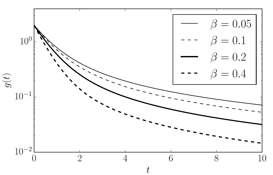
Fig. 23 Convolution kernel function \(g(t) = {\cal L}^{-1} [G(s)]\) of Eq. (46) as computed by the Weideman inversion method. Plots are shown for \(s_0=2\) and four values of \(\beta\).

Summary of inversion method

In these notes we have outlined a modification to the Weideman method for numerical calculation of the inverse Laplace transform. The modified method is suitable for calculating the time-domain loudspeaker response and can be implemented in only a few lines of code. The complete algorithm is summarized by Eqs. (37), (40), (41) and (42). Importantly, it can be applied to nonstandard frequency-domain response functions containing branch cuts, as encountered in advanced transducer models with semi-inductance in the motor or viscoelasticity in the suspension. Alternatively, this method can be used as a simple and rapid method to compute the time-domain response for simple polynomial response functions.

Appendices

Simplification of the Ritter 3PC compliance model

In Eq. (13) of a paper by Ritter and Agerkvist [RA10], the viscoelastic compliance contains a logarithmic term that is expressed as

\[\log_{10} \left[ \frac{i \omega \tau_\mathrm{min} e^{-i \beta}}{\sqrt{1+\omega^2\tau_\mathrm{min}^2}} \right] \; .\]

In this expression, \(\beta=\tan^{-1}(\tau_\mathrm{min} \omega)\) is the phase angle. We remark that Ritter’s \(\beta\) is unrelated to \(\beta\) in these notes. By defining \(s_0 \doteq 1/\tau_\mathrm{min}\), setting \(s=i\omega\), and expanding the complex exponential, we can rewrite this as

\[\log_{10} \left[ \frac{(s/s_0)}{\sqrt{1-s^2/s_0^2}} \left( \cos\beta - i \sin\beta\right) \right] \; .\]

Next, using the identities

\[\sin\beta = \frac{\omega/s_0}{\sqrt{1+\omega^2/s_0^2}} \; , \quad \cos\beta = \frac{1}{\sqrt{1+\omega^2/s_0^2}} \; ,\]

which follow from \(\tan\beta = \omega/s_0\), we can write the argument as

\[\log_{10} \left[ \frac{(s/s_0) \left( 1-s/s_0 \right)}{1-s^2/s_0^2} \right] = \log_{10} \left( \frac{s}{s+s_0} \right) \; ,\]

which is the argument used in Eq. (43).

Sample Python code for inverse transform

The following Python code implements the algorithm of Eq. (37) as applied to the closed box response function of Eq. (29).

import numpy as np
import time

def y(s):
    qts = 0.5
    alpha = 0.0
    y = s**2/(s**2+s/qts+1+alpha)
    return y
              
def step():

   #------------------------------------------------------------
   # Some adjustable settings

   # Number of time points
   nt = 400

   # Initial number of integration nodes along parabola
   N0 = 16

   # Max(ws*t) = total integration time (t_max in AES paper)
   tmax = 8.0
   #------------------------------------------------------------

   mu_c = max(1,h)
   t_c = np.pi*N0/(12*mu_c)

   # Pack points closer to t=0
   tvec = tmax*np.linspace(1e-4,1.0,nt)**2
   svec = np.zeros(nt)
   
   for j in range(nt):

      t = tvec[j]

      if t<t_c:
         mu = np.pi*N0/(12.0*t)
         N = N0
      else:
         mu = mu_c
         N = np.ceil(N0*t/t_c).astype('int')

      d = 3.0/N
  
      # Vectorize over contour sum
      u = d*np.arange(-N,N+1)
      s = mu*(1j*u+1)**2
      dsdu = 2.0*mu*(1j-u)
      step = np.sum(np.imag(np.exp(s*t)*y(s)/s*dsdu))*d/(2*np.pi) 
      
      # step response
      svec[j] = step

   return tvec,svec

t,s = step()

exact = np.exp(-t)*(1-t)
for i,t0 in enumerate(t):
    print('{:.3f} {:.4f} {:.4f}'.format(t0,p[i],exact[i]))