Classic Vented Alignments

In classical loudspeaker theory from the 1960s onwards, the concept of alignments was developed to provide a systematic prescription for choosing box volume and port tuning to yield a target low-frequency response. While the theory is not exact, it offers numerous benefits including insight into the choice between low frequency extension versus group delay (phase distortion). A brief overview of the alignments discussed here and supported in Speakerbench is given in the Summary section at end of this page.

Alignment source code

All the plots and data output shown on this page were generated using the Speakerbench python alignment library. That library and all software (including these webpages) is freely-available

• Source code at GitHub speakerbench repository.

• Download ZIP archive

• Download TGZ archive

$ unzip libalignment.zip
$ python print_qt.py
$ python print_c4.py
$ python print_qa.py
$ python print_quasi.py

Within the ZIP file is a Python library of functions (libalignment.py), which is used in code samples throughout this chapter.

General framework

To facilitate choosing the box volume and vent tuning, Speakerbench will propose values based on standard 4^th-order bass-reflex alignments. These alignments are particular types of 4^th-order high-pass filters. Following Small [Sma73b] (Eq. 57) we can write the normalized response function as

(22)\[G_\mathrm{H}(s) = \frac{s^4}{s^4 + a_1 s^3 + a_2 s^2 + a_3 s + 1} \; ,\]

where \(s = j \omega / \omega_0\) is the dimensionless complex frequency variable normalized to \(\omega_0 \doteq \sqrt{\wb\ws} = \sqrt{h} \, \ws\). In the first part of his article series, Small [Sma73b] (Eqs. 22-24) writes the lossy box filter coefficients as

(23)\[\begin{split}\displaystyle a_1 & = \frac{\ql + h \: \qts}{\sqrt{h} \: \ql \: \qts} \\ a_2 & = \frac{h + (\alpha + 1 + h^2) \: \ql \: \qts}{h \: \ql \: \qts} \\ a_3 & = \frac{h \: \ql + \qts}{\sqrt{h} \: \ql \: \qts} \; ,\end{split}\]

where \(\ql\) is the leakage-loss \(Q\) of the box and \(\qts\) is the total \(Q\) of the driver. Here, \(h = \wb/\ws\) is the system tuning ratio and \(\alpha =\vas/\vb\) is the ratio of the compliance volume to the box volume. We remark that the coefficients are approximate and neglect myriad other terms which appear in a more comprehensive model of a vented box. These missing terms would represent more complex losses in the box and in the driver suspension system, driver inductance and semi-inductance, and so on. It is generally accepted that \(\ql\) does not represent a true leakage loss. Rather it is an approximate total loss which is dominated by driver losses not accounted for in the standard Thiele-Small theory. These losses are included in the advanced model and thus we recommend setting \(\ql \geq 100\) in this case.

In the definition of \(\omega_0\), \(\ws\) is the driver resonant frequency and \(\wb\) is the vent resonant frequency. This normalization is equivalent to setting \(T_0=1\) in Small’s expressions. The magnitude-versus-frequency behavior is also given in Small [Sma73b] (Eqs. 58 and 59) facilitated by the use of the squared modulus technique, which we reproduce here as

\[\left| G_\mathrm{H}(i\omega) \right|^2 = \frac{\omega^8}{\omega^8 + A_1 \omega^6 + A_2 \omega^4 + A_3 \omega^2 + 1} \; ,\]

where

\[\begin{split}A_1 & = a_1^2-2 a_2 \; , \\ A_2 & = a_2^2+2-2 a_1 a_3 \; , \\ A_3 & = a_3^2-2 a_2 \; .\end{split}\]

A note about series resistance

The driver Q is given by

\[\frac{1}{\qts} = \frac{1}{\qms} + \frac{1}{\qes} \; .\]

Here, we have the electrical and mechanical Q values

\[\begin{split}\qms & = \frac{\mms}{\rms} \, \ws \\ \qes & = \frac{\mms}{\rme} \, \ws\end{split}\]

where \(\rme\) is the electrical DC resistance \(\re\) converted to the mechanical side. The electrical damping depends on the electrical resistance of the driver voice coil \(\re\) as well as any added electrical resistance \(R_\mathrm{S}\) in series with the driver including the output resistance \(R_g\) of the voltage source (amplifier), and we may name this \(R_\mathrm{MES}\)

\[R_\mathrm{MES} = \frac{\bls}{\re + R_\mathrm{S}} \; .\]

When you enable the optional filter in the Speakerbench box mode, and apply a series resistance, the modified value \(Q_\mathrm{T,R_S}\) is calculated in Speakerbench and displayed in the INFO tab.

\[Q_\mathrm{T,R_S} = \frac{\mms}{R_\mathrm{MES} + \rms} \, \ws\]

This value is what Speakerbench uses for response calculations (and in the alignment chart). The second-order response function (see Second-order alignments) becomes:

\[G_\mathrm{H}(u) = \frac{u^2}{\displaystyle u^2 + \frac{u}{Q_\mathrm{T,R_S}} + 1 + \alpha} \; .\]

Discrete alignments

A discrete bass reflex alignment means we need to select a driver with a specific \(\qts\) value and match that with a specific box volume and port tuning frequency to obtain the unique discrete alignment. Two popular classic discrete alignments are the Butterworth (B4) and Bessel (BL4) ones. In addition, Thiele [Thi74] defined the Inter-Order Butterworth (IB4) discrete alignment around 1974. In these notes we further discuss the so-called Linkwitz-Riley (LR4) and Critically Damped (CD4) discrete alignments. Each discrete alignment defines a specific 4^th-order filter with fixed coefficients \((a_1,a_2,a_3)\) along with properties that are broadly suitable for vented aligments. The coefficients are

Butterworth B4

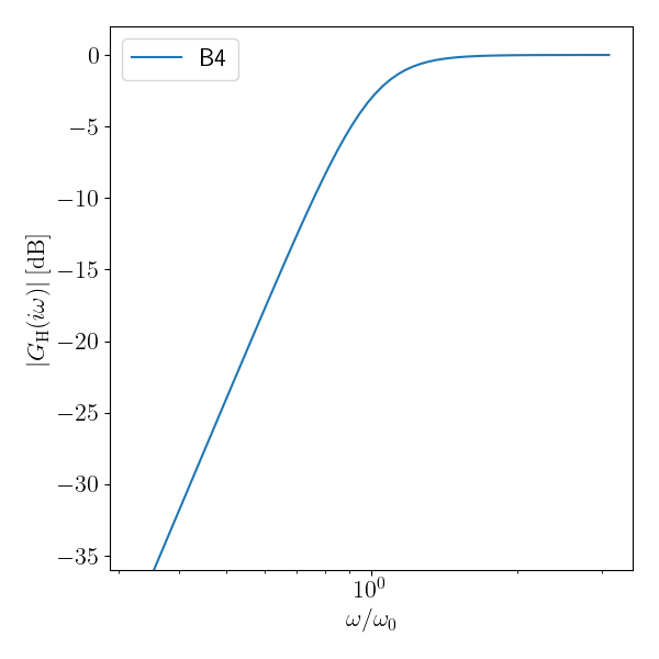
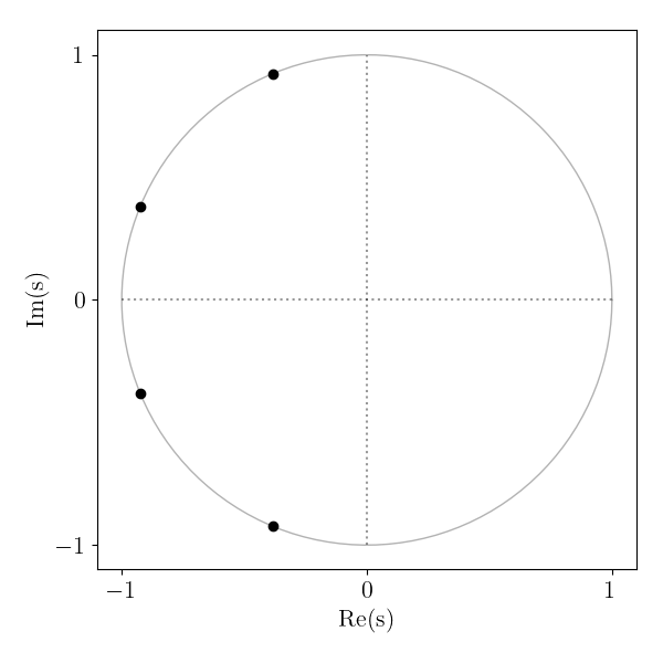
Fig. 14 B4 amplitude and poles.

In the limit of no losses, the Butterworth (B4) response corresponds to

\[\begin{split}\qts & = \cos\frac{3\pi}{8} \simeq 0.3827 \\ h & = 1 \\ \alpha & = \sqrt{2} \simeq 1.414\end{split}\]

The Butterworth filter was introduced in 1930 by Stephen Butterworth [But30]. It offers a maximally-flat frequency response (with no ripple in the passband) with the sharpest knee point towards the roll-off region and thus the most extended bandwidth. In relation to bass reflex loudspeakers, B4 was a very popular target response for many years, and several (non-discrete) alignment families ultimately develops from B4. The filter coefficients depend on cosines of the pole locations, and have the exact values

\[a_1 = 2 \cos\frac{\pi}{8} + 2 \cos\frac{3\pi}{8} \qquad a_2 = 2+4 \cos\frac{\pi}{8} \cos\frac{3\pi}{8} \qquad a_3 = a_1\]

The remarkable vanishing of all coefficients \((A_1,A_2,A_3)\) when calculating the squared modulus demonstrates the maximally-flat property via

\[\left| G_\mathrm{H}(i\omega) \right|^2 = \frac{\omega^8}{\omega^8 + 1} \; ,\]

Linkwitz-Riley LR4

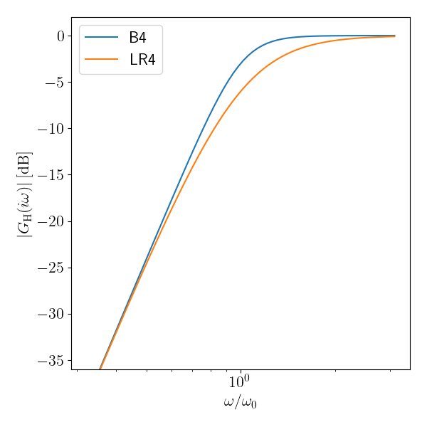
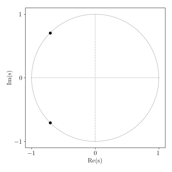
Fig. 15 LR4 amplitude and poles (two double poles).

In the limit of no losses, the Linkwitz-Riley (LR4) response corresponds to

\[\begin{split}\qts & = 1/\sqrt{8} \simeq 0.3536 \\ h & = 1 \\ \alpha & = 2\end{split}\]

In 1976, some years after Thiele’s work, Linkwitz-Riley filters for use in electronic crossover design were described by Siegfried H. Linkwitz in a series of articles [Lin76, Lin78]. Linkwitz obtained the 2^nd- and 4^th-order filters by squaring the 1^st- and 2^nd-order Butterworth filters, respectively. In the 4^th-order case,

\[G_\mathrm{H}(s) = \frac{ s^4 } { \left(s^2 + \sqrt{2} s + 1 \right)^2 } \; .\]

An important property of the combined high-pass and low-pass sections is that the resulting crossover sums to unit magnitude, with the outputs in phase at the crossover frequency. Linkwitz originally proposed filters with these characteristic for solving lobing issues with noncoincident transducers. Of course, the application to crossovers is unrelated to bass-reflex design, which may partly explain why the literature seems to contain no recorded use of the Linkwitz-Riley filter as a discrete target alignment. In relation to bass reflex alignment, LR4 exhibits desirable features like fast settling time (controlled impulse response) similar to Bessel BL4 but with a more extended frequency response. The response coefficients are

\[a_1 = \sqrt{8} \simeq 2.828 \qquad a_2 = 4 \qquad a_3 = a_1 \; .\]

Although the Linkwitz-Riley alignment was never explicitly mentioned anywhere prior to the article in Voice Coil Magazine, it is a specific instance of the Boombox BB4 family of alignments for \(\zeta = 1/\sqrt{2}\). The LR4 alignment was first presented in the Voice Coil Magazine, June 2024. Later the article became Open Access when AudioXpress released an LR4 article.

Inter-Order Butterworth IB4

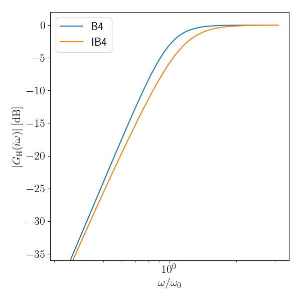
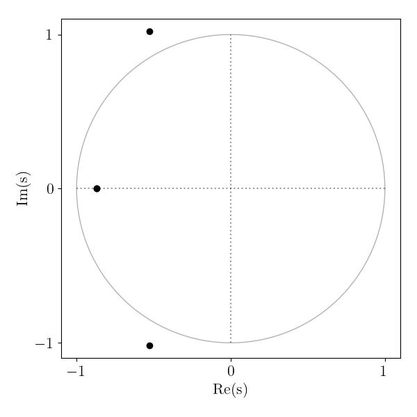
Fig. 16 IB4 amplitude and poles (the pole on the x-axis is a double pole).

In the limit of no losses, the Inter-order Butterworth (IB4) response corresponds to

\[\begin{split}\qts & \simeq 0.3398 \\ h & \simeq 1.106 \\ \alpha & \simeq 2.107\end{split}\]

Thiele defined IB4 as a combination of a general second-order filter and two identical first-order filters [Thi74]

\[G_\mathrm{H}(s) = \frac{ s^4 } { \left( s^2 + \lambda s + \beta \right) \left(s + 1\right)^2 } \; ,\]

where \(\lambda\) and \(\beta\) are free parameters to be chosen according to the flatness condition

(24)\[\left\| \left( s^2 + \lambda s + \beta \right) \left(s + 1\right)^2 \right\|^2 = 1 + 4 \omega^6 + 3 \omega^8 \; .\]

In these equations, \(s = i\omega\) and \(\omega\) are not yet properly normalized. Note that on the righthand side of (24), the coefficients of \(\omega^2\) and \(\omega^4\) have been set to zero. This implies that IB4 is a special case of QB3 (referred to in this work as B4Q). By solving (24) we can deduce the required coefficients

\[\begin{split}\lambda & = \sqrt{2 \left(\sqrt{3} - 1\right)} \; , \\ \beta & = \sqrt{3} \; . \\\end{split}\]

Then, bringing the high-pass filter into canonical form, the polynomial coefficients \(a_1\), \(a_2\), and \(a_3\) are expressed as

\[a_1 = \frac{2+\lambda}{\beta^{1/4}} \qquad a_2 = \frac{1+2\lambda+\beta}{\beta^{1/2}} \qquad a_3 = \frac{\lambda+2\beta}{\beta^{3/4}}\]

The Inter-Order Butterworth (IB4) alignment is rarely talked about. It was mentioned briefly by Richard Small [Sma73b]. Bullock [BullockIII81] published a table for this discrete alignment, and the tables are reproduced in The Loudspeaker Design Cookbook by Vance Dickason. The IB4 alignment was first presented in Voice Coil Magazine, July 2024. Later the article became Open Access when AudioXpress released an IB4 article.

Bessel BL4

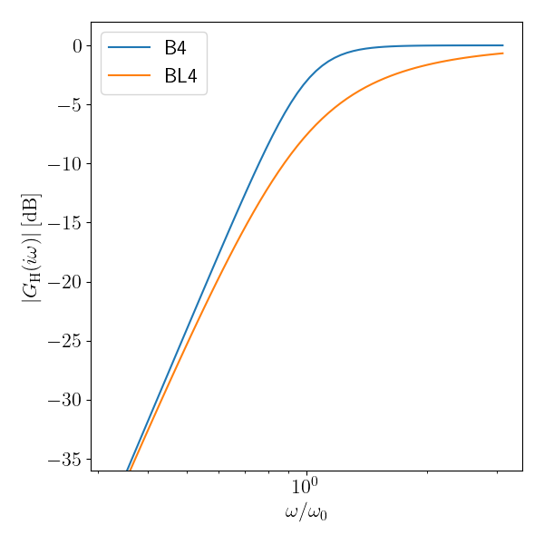
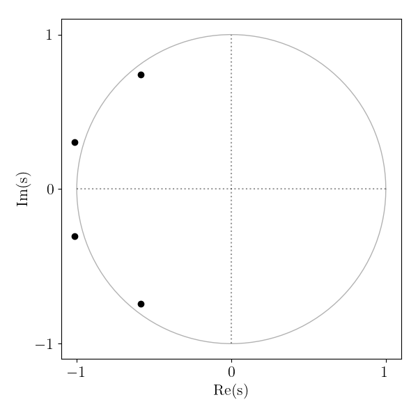
Fig. 17 BL4 amplitude and poles.

In the limit of no losses, the Bessel response corresponds to

\[\begin{split}\qts & \simeq 0.3162 \\ h & \simeq 0.9759 \\ \alpha & \simeq 2.333\end{split}\]

The filter coefficients can be written in terms of the 4^th-order Bessel polynomial

\[y_4(x) = 105 x^4 + 105 x^3 + 45 x^2 + 10 x + 1 \; .\]

Bringing the high-pass response function into the canonical form (22) shows that

\[a_1 = \frac{105}{105^{3/4}} \qquad a_2 = \frac{45}{105^{1/2}} \qquad a_3 = \frac{10}{105^{1/4}} \; .\]

Bessel polynomials arise in the theory of Bessel functions and are named after Friedrich Wilhelm Bessel (1784-1846) in tribute to his systematic study of Bessel’s differential equation. The practical application to filters was worked out by W.E. Thomson in 1949 in a scientific article titled Delay Networks Having Maximally Flat Frequency Characteristics. Thomson described this filter function applied to delay lines. A frequency range with flat group delay implies nearly linear phase response and hence minimal phase distortion of the signal. Low-pass Bessel filters are characterized by the fastest settling time and maximally flat group delay of the form

\[\tau_g = -\frac{d\phi}{d\omega} \sim 1 + O(\omega^8)\]

Critically damped CD4

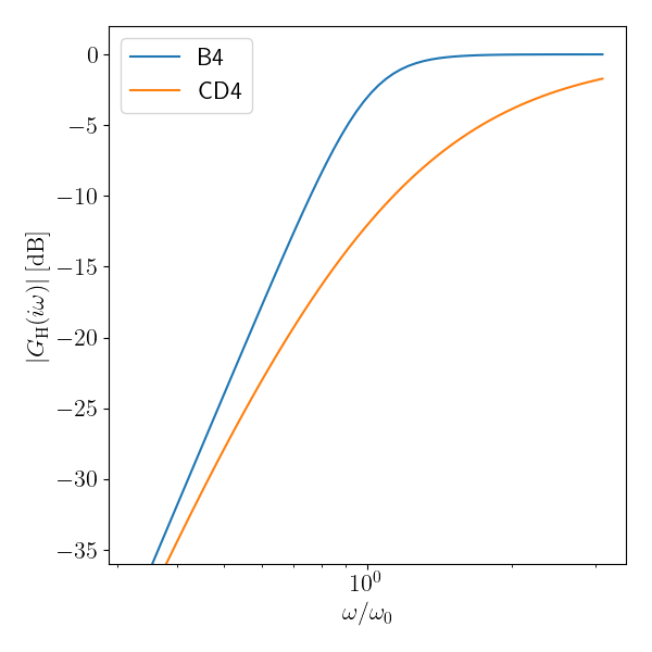
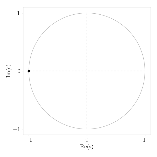
Fig. 18 CD4 amplitude and poles (one quadruple pole).

In the limit of no losses, the critically damped response corresponds to

\[\begin{split}\qts & = 0.25 \\ h & = 1 \\ \alpha & = 4\end{split}\]

A critically-damped response has all 4 poles at \(s=-1\), such that the response function is

\[G_\mathrm{H}(s) = \frac{ s^4 } { (s + 1)^4 } = \frac{s^4}{s^4 + 4 s^3 + 6 s^2 + 4 s + 1} \; .\]

Because of the reality of the poles, the step response for a CD4 aligment is non-oscillatory (no overshoot). Thus, CD4 is the most extended frequency response of all alignments with no overshoot. In relation to bass reflex design, however, this alignment is not commonly used due to the early roll-off in the frequency response. We remark that CD4 is also a special case of the Boombox BB4 family for \(\zeta = 1\). CD4 is also equivalent to two cascaded 2^nd-order filters each with \(\qfilt = 0.5\), where \(\qfilt\) is the filter-Q

\[s^2+s/\qfilt+1 \; .\]

In the lossless case \(\ql \rightarrow \infty\), the CD4 alignment corresponds to a driver with \(\qts = 0.25\). A discussion of the CD4 alignment was presented in Voice Coil Magazine in August 2024. Later the article became Open Access when AudioXpress released a CD4 article.

Comparison

Fig. 19 shows the (normalized) amplitude response and group delay of the above mentioned discrete alignments.

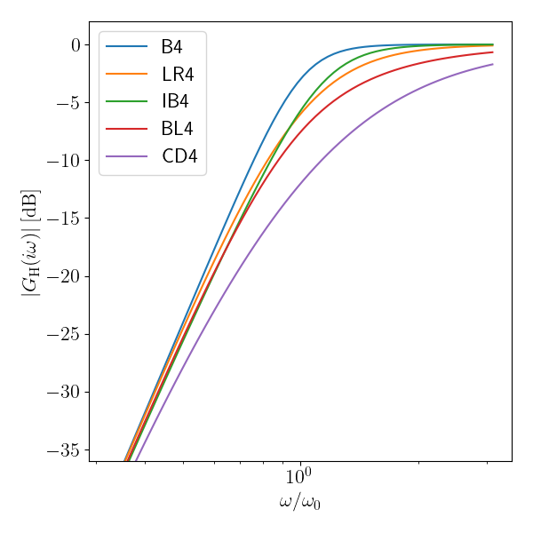
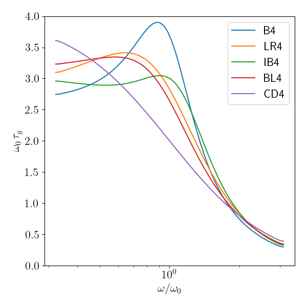
Fig. 19 The normalized amplitude response \(|G_\mathrm{H}|\) (left) and group delay \(\omega_0 \tau_g = -d\phi/d\omega\) (right) of the five discrete alignments.

Note: These graphs are not normalized relative to the driver’s resonance frequency, but \(\omega_0 \doteq \sqrt{\wpb \, \ws} = \sqrt{h} \, \ws\). Below, we tabulate each of the five discrete alignments as a function of the enclosure loss \(\ql\). The python source code used is also shown.

CLICK HERE to expand discrete alignment source code

import numpy as np
from libalignment import *

Ql_vec = ['inf',100,50,10,7]

print('             B4                    LR4                   IB4                   BL4                   CD4        ' )
print(' Ql     Qt    h    alpha      Qt    h    alpha      Qt    h    alpha      Qt    h    alpha      Qt    h    alpha ')
print('---  --------------------  --------------------  --------------------  --------------------  --------------------')

for Ql in Ql_vec:
   if Ql == 'inf':
      ql = 0.0
   else:
      ql = 1/Ql

   a1,a2,a3 = coef('B4')
   Qt1,h1,alpha1 = qtsolve(a1,a2,a3,ql)
   a1,a2,a3 = coef('LR4')
   Qt2,h2,alpha2 = qtsolve(a1,a2,a3,ql)
   a1,a2,a3 = coef('IB4')
   Qt3,h3,alpha3 = qtsolve(a1,a2,a3,ql)
   a1,a2,a3 = coef('BL4')
   Qt4,h4,alpha4 = qtsolve(a1,a2,a3,ql)
   a1,a2,a3 = coef('CD4')
   Qt5,h5,alpha5 = qtsolve(a1,a2,a3,ql)
  
   print('{:3}  {:.4f} {:.4f} {:.4f}  {:.4f} {:.4f} {:.4f}  {:.4f} {:.4f} {:.4f}  {:.4f} {:.4f} {:.4f}  {:.4f} {:.4f} {:.4f}'.
         format(Ql,
                Qt1,h1,alpha1,
                Qt2,h2,alpha2,
                Qt3,h3,alpha3,
                Qt4,h4,alpha4,
                Qt5,h5,alpha5
                ))
                

             B4                    LR4                   IB4                   BL4                   CD4        
 Ql     Qt    h    alpha      Qt    h    alpha      Qt    h    alpha      Qt    h    alpha      Qt    h    alpha 
---  --------------------  --------------------  --------------------  --------------------  --------------------
inf  0.3827 1.0000 1.4142  0.3536 1.0000 2.0000  0.3398 1.1064 2.1071  0.3162 0.9759 2.3333  0.2500 1.0000 4.0000
100  0.3842 1.0000 1.3882  0.3548 1.0000 1.9718  0.3409 1.1072 2.0759  0.3172 0.9757 2.3022  0.2506 1.0000 3.9601
 50  0.3856 1.0000 1.3624  0.3561 1.0000 1.9438  0.3421 1.1079 2.0450  0.3182 0.9756 2.2713  0.2513 1.0000 3.9204
 10  0.3979 1.0000 1.1629  0.3665 1.0000 1.7272  0.3518 1.1146 1.8042  0.3266 0.9743 2.0311  0.2564 1.0000 3.6100
  7  0.4048 1.0000 1.0613  0.3724 1.0000 1.6163  0.3572 1.1185 1.6803  0.3312 0.9735 1.9076  0.2593 1.0000 3.4490

Modification of discrete alignments

For the five discrete alignments described above, \(\qts\) is not a free parameter. This suggests that a particular alignment cannot be achieved with an arbitrary driver. Thus we are faced with the problem of misalignment.

misalignment

If the driver \(\qts\) does not match that required by your desired target alignment, the driver is said to be misaligned.

In the sections below we will describe three approaches to deal with misalignment.

Method 1: Ignorance

The simplest solution is to ignore the fact that the driver \(\qts\) is far from the target \(\qts\). This we call the method of ignorance, because you ignore the fact that \(\qts\) is wrong. Speakerbench denotes this approach by adding a trailing ‘i’ to the name: B4i, LR4i and BL4i. In this case, the suggested \(h\) and \(\alpha\) are unaffected by the driver \(\qts\) (the fact that \(\qts\) is not correct is ignored). The method of ignorance is not recommended for actual use, but is included for reference. Despite the name, we suspect the method was commonly used in the past.

Method 2: Compliance alteration

A second and better approach to handling misalignment (i.e., approximating a desired discrete alignment for which the driver \(\qts\) does not match the alignment \(\qts\)) is compliance alteration. In this case we imagine that the driver compliance starts out at a value for which the driver \(\qts\) matches the alignment \(\qts\). A box and port are designed with the required \(h\) and \(\alpha\). We call these the reference values: \(Q_\mathrm{TS,ref}\), \(\alpha_\mathrm{ref}\) and \(h_\mathrm{ref}\). Then, overnight, the suspension softens or hardens such that the driver obtains the value \(\qts\). Compliance alteration then shifts \(\alpha\) and \(h\) according to

\[\begin{split}\alpha & = \alpha_\mathrm{ref} \left( \frac{Q_\mathrm{TS,ref}}{\qts} \right)^2 \; , \\ h & = h_\mathrm{ref} \left( \frac{Q_\mathrm{TS,ref}}{\qts} \right) \; .\end{split}\]

In Speakerbench, when we apply this method, the alignment acronym is followed by CA as in B4CA, LR4CA and BL4CA. Below we tabulate sample alignments for \(\ql = 10\)

CLICK HERE to expand compliance alteration source code

import numpy as np
from libalignment import *

Ql = 10
Qt_vec = [0.30,0.32,0.34,0.36,0.38,0.40]

h0     = {}
alpha0 = {}

print('            B4CA                  LR4CA                 IB4CA                 BL4CA                 CD4CA        ')
print(' Ql     Qt    h    alpha      Qt    h    alpha      Qt    h    alpha      Qt    h    alpha      Qt    h    alpha ')
print('---  --------------------  --------------------  --------------------  --------------------  --------------------')

ql = 1/Ql
for Qt in Qt_vec:
   for align in ['B4','LR4','IB4','BL4','CD4']:
      a1,a2,a3 = coef(align)
      Qtref,href,aref = qtsolve(a1,a2,a3,ql)
      h0[align],alpha0[align] = casolve(Qt,Qtref,href,aref)
 
   print('{:3}  {:.4f} {:.4f} {:.4f}  {:.4f} {:.4f} {:.4f}  {:.4f} {:.4f} {:.4f}  {:.4f} {:.4f} {:.4f}  {:.4f} {:.4f} {:.4f}'.
         format(Ql,
                Qt,h0['B4'],alpha0['B4'],
                Qt,h0['LR4'],alpha0['LR4'],
                Qt,h0['IB4'],alpha0['IB4'],
                Qt,h0['BL4'],alpha0['BL4'],
                Qt,h0['CD4'],alpha0['CD4'],
                ))
                

            B4CA                  LR4CA                 IB4CA                 BL4CA                 CD4CA        
 Ql     Qt    h    alpha      Qt    h    alpha      Qt    h    alpha      Qt    h    alpha      Qt    h    alpha 
---  --------------------  --------------------  --------------------  --------------------  --------------------
 10  0.3000 1.3264 2.0458  0.3000 1.2217 2.5779  0.3000 1.3070 2.4808  0.3000 1.0605 2.4066  0.3000 0.8547 2.6372
 10  0.3200 1.2435 1.7981  0.3200 1.1453 2.2657  0.3200 1.2253 2.1804  0.3200 0.9943 2.1152  0.3200 0.8013 2.3178
 10  0.3400 1.1703 1.5928  0.3400 1.0780 2.0070  0.3400 1.1532 1.9314  0.3400 0.9358 1.8736  0.3400 0.7541 2.0531
 10  0.3600 1.1053 1.4207  0.3600 1.0181 1.7902  0.3600 1.0892 1.7228  0.3600 0.8838 1.6712  0.3600 0.7123 1.8314
 10  0.3800 1.0471 1.2751  0.3800 0.9645 1.6067  0.3800 1.0318 1.5462  0.3800 0.8373 1.4999  0.3800 0.6748 1.6437
 10  0.4000 0.9948 1.1508  0.4000 0.9163 1.4501  0.4000 0.9803 1.3954  0.4000 0.7954 1.3537  0.4000 0.6410 1.4834

Compliance Alteration was first presented in Voice Coil Magazine from October 2024. Later, the article became Open Access when AudioXpress released an Compliance Alteration article. The method can be applied to any desired discrete target alignment. This method is particularly interesting if your driver \(\qts\) is a bit too high, because with the compliance alteration technique, the box calculation is then treated as if the suspension is a bit too stiff. Fortunately, the driver suspension will experience aging (or burn-in) over time and will soften. When this happens, the provided equations dictate that your system will, over time, move toward the desired target response, and if softened enough to reach \(Q_\mathrm{TS,ref}\), the system response will match the target without any error. If the softening does not happen, the system response will deviate slightly from the target.

Method 3: Generalized quasi-alignment

In a design process based on alignments, we consider \((\ql,\qts)\) as given inputs and \((\alpha,h)\) as output parameters to be computed by the alignment. Since we have two free parameters, it follows that we can specify only two of the three values \((A_1,A_2,A_3)\). The approach taken is to relax (i.e., ignore) the condition on \(A_3\); that is, we match the behaviour in the pass-band \((A_1)\) and mid-band \((A_2)\) but not the stop-band \((A_3)\). This is described in more detail for so-called QB3 (although we prefer B4Q because the order of the filter is 4) lossless case by Benson [Ben93] (page 188).

By defining \(G = \left( \alpha+1+h^2 \right)/h\), we can rewrite these two conditions as

\[\begin{split}\begin{eqnarray} A_1 &=& \frac{q^2}{h} - 2G + \epsilon^2 q^2 h \; , \\ A_2 &=& \left( G + \epsilon q^2 \right)^2 + 2-2q^2\left[ 1+\epsilon^2+\epsilon (h+1/h) \right] \; . \end{eqnarray}\end{split}\]

where \(q = 1/\qts\) and \(\epsilon = \qts/\ql \ll 1\) is a small parameter.

Recursive solution

In the limit \(\epsilon = 0\), we can solve explicitly for \((G,h)\), and this uniquely determines \((\alpha,h)\). However, an explicit solution is not possible in the case \(\epsilon > 0\). But since \(\epsilon\) is small, we expect the following recursion to converge in a few iterations:

\[\begin{split}\begin{eqnarray} G &=& -\epsilon q^2 + \sqrt{A_2-2+2q^2 \left[ 1+\epsilon^2+\epsilon\left(h+1/h\right)\right]} \\ h &=& \frac{q^2}{2G + A_1-\epsilon^2 q^2 h} \end{eqnarray}\end{split}\]

Once converged, we can obtain \(\alpha\) according to

\[\alpha = Gh-\left(1+h^2\right)\]

Finally, note that by setting \(\epsilon=0\) above we obtain the lossless solution explicitly.

CLICK HERE to expand quasi-alignment source code

import numpy as np
from libalignment import *

Ql = 10
Qt_vec = [0.30,0.32,0.34,0.36,0.38,0.40]

h0     = {}
alpha0 = {}

print('             B4Q                  LR4Q                  IB4Q                 BL4Q                   CD4Q         ')
print(' Ql     Qt    h    alpha      Qt    h    alpha      Qt    h    alpha      Qt    h    alpha      Qt    h    alpha ')
print('---  --------------------  --------------------  --------------------  --------------------  --------------------')

ql = 1/Ql
for Qt in Qt_vec:
   for align in ['B4','LR4','IB4','BL4','CD4']:
      a1,a2,a3 = coef(align)
      A1 = a1**2-2*a2
      A2 = a2**2+2-2*a1*a3
      h0[align],alpha0[align] = quasi(Ql,Qt,A1,A2)
 
   print('{:3}  {:.4f} {:.4f} {:.4f}  {:.4f} {:.4f} {:.4f}  {:.4f} {:.4f} {:.4f}  {:.4f} {:.4f} {:.4f}  {:.4f} {:.4f} {:.4f}'.
         format(Ql,
                Qt,h0['B4'],alpha0['B4'],
                Qt,h0['LR4'],alpha0['LR4'],
                Qt,h0['IB4'],alpha0['IB4'],
                Qt,h0['BL4'],alpha0['BL4'],
                Qt,h0['CD4'],alpha0['CD4'],
                ))
                

             B4Q                  LR4Q                  IB4Q                 BL4Q                   CD4Q         
 Ql     Qt    h    alpha      Qt    h    alpha      Qt    h    alpha      Qt    h    alpha      Qt    h    alpha 
---  --------------------  --------------------  --------------------  --------------------  --------------------
 10  0.3000 1.2890 2.9022  0.3000 1.2294 3.0517  0.3000 1.2890 2.9022  0.3000 1.0736 2.6230  0.3000 0.8032 2.3073
 10  0.3200 1.2146 2.4150  0.3200 1.1505 2.5657  0.3200 1.2146 2.4150  0.3200 0.9972 2.1634  0.3200 0.7320 1.8855
 10  0.3400 1.1493 2.0109  0.3400 1.0808 2.1629  0.3400 1.1493 2.0109  0.3400 0.9301 1.7839  0.3400 0.6700 1.5387
 10  0.3600 1.0918 1.6719  0.3600 1.0188 1.8253  0.3600 1.0918 1.6719  0.3600 0.8705 1.4670  0.3600 0.6155 1.2502
 10  0.3800 1.0409 1.3846  0.3800 0.9631 1.5396  0.3800 1.0409 1.3846  0.3800 0.8172 1.1999  0.3800 0.5673 1.0079
 10  0.4000 0.9955 1.1389  0.4000 0.9130 1.2957  0.4000 0.9955 1.1389  0.4000 0.7694 0.9728  0.4000 0.5244 0.8025

In Speakerbench, when we apply this method, the alignment acronym is followed by Q as in B4Q, LR4Q and BL4Q. Thus, B4Q in Speakerbench is the same as what is known in classical theory as the QB3 alignment. We remark that Bullock [BullockIII81] defines SQB3 as a subset of QB3 for drivers with \(0.56 > \qts > 0.4\).

Alignment families

Beyond discrete aligments, for which \((a_1,a_2,a_3)\) have explicit numerical values, well-known alignment families exist for which \((a_1,a_2,a_3)\) depend upon a free parameter. The term alignment family is derived from the mathematical definition of a family of response curves. An alignment family allows one to cover a range of driver \(\qts\) values rather than just a single value. The B4Q quasi-alignment described above is in the loudspeaker industry considered an alignment family. Small and others refer to this family as QB3 (references).

Boombox BB4

The Boombox family of alignments was first described in a convention article by W.J.J. Hoge in 1976, later in the JAES [Hog77]. This alignment is relatively simple, and cascades two identical 2^nd-order polynomials according to

\[G(s) = \frac{ s^4 } { \left( s^2 + 2 \, \zeta \, s + 1 \right)^2 }\]

where the free parameter \(\zeta\) is the damping ratio, which is directly related to the driver’s \(\qts\)-value. For a chosen \(\qts\) and \(\ql\), we have

\[\begin{split}\zeta & = \frac{1}{4} \left( \frac{1}{\qts} + \frac{1}{\ql} \right) \\ \alpha & = \frac{1}{4} \left( \frac{1}{\qts} - \frac{1}{\ql}\right)^2 \\ h & = 1\end{split}\]

Bullock [BullockIII81] presents tables for \(\ql \geq 3\)-value, which is exceptionally lossy and seems unlikely for practical use. Hoge was focused on a suitable alignment for instrument loudspeakers, e.g., for electric guitars, and was seeking a bass reflex alignment option for the high \(\qts\) drivers of the time that could provide an alternative to Chebyshev C4. Choosing to cascade two identical 2^nd-order polynomials gives double poles with reasonably fast settling time for an impulse. Unfortunately, this alignment creates a peak before roll-off which led Hoge to satirically name it the Boombox alignment, or BB4. Hoge only defined the BB4 alignment for driver \(\qts\) above roughly 0.37, and he identified the peak with \(\ql = 7\) for a driver \(\qts = 0.72\) to be around +6 dB. For high \(\qts\) drivers, the peak becomes large, which you might accept in favor of the impulse stopping quicker than a similar peaky Chebyshev response. Besides, the single peak of a BB4 alignment is easier to equalize electronically, than the ripples of a Chebyshev alignment. On the other hand, a Chebyshev alignment with a similar driver \(\qts\) results in 1.3 - 1.4 dB ripple. Finally, when driver \(\qts\) is this high, one may consider a large closed box. Bullock realized that the equations also work well for drivers with lower \(\qts\), and in this case there is no peak in the frequency response. He coined the term Sub-Boombox for these alignments, or SBB4, and his tables go as low as \(\qts = 0.20\). It is therefore reasonable to say that the BB4-SBB4 alignment works for driver \(\qts\) in the range of 0.20-0.72, although mathematically it can be applied outside these limits. Note finally that both LR4 and CD4 are special cases of BB4 for \(\zeta = 1/\sqrt{2}\) and \(\zeta = 1\) respectively.

Transitional B4-LR4

Speakerbench supports a so-called Transitional B4-LR4 alignment family, which moves smoothly between Butterworth B4 and Linkwitz-Riley LR4. The construction is fairly trivial by comparing locations of LR4 and B4 poles. We can write a one-parameter family of alignments that contains both B4 and LR4 as specific cases using

\[\begin{split}a_1 &= \sqrt{8} \cos\epsilon \\ a_2 &= 4 \cos^2 \epsilon \\ a_3 &= a_1\end{split}\]

where \(\epsilon\) is an angle in the range \(0 \leq \epsilon \leq \pi/8\). Evidently

\[\cos\epsilon = \frac{1}{\sqrt{8}} \left( \frac{1}{\qts} + \frac{1}{\ql} \right)\]

Importantly, \(\epsilon = 0\) gives LR4 and \(\epsilon = \pi / 8\) gives B4. In general, the four poles of the response function lie on the unit circle at

\[\begin{split}\theta & = \frac{3\pi}{4} \pm \epsilon \\ \theta & = -\frac{3\pi}{4} \pm \epsilon\end{split}\]

To the best of our knowledge, the concept of Transitional Alignments was never explored in relation to loudspeaker (Bass Reflex) boxes until it was presented in the Voice Coil Magazine, September 2024. Later the article became Open Access when AudioXpress released an online Transitional alignment article. Notably, R.M. Golden and J.F. Kaiser [GK71] described the roots of normalized Butterworth and Bessel-Thomson low-pass transfer functions, from which Small [Sma73b] derived the polynomial coefficients of the fourth-order highpass Bessel alignment. Golden and Kaiser also described a transitional filter design where a chosen balance between the two is realized.

With the calculated transition from LR4 to B4, we have obtained a subtle improvement over continuing with the Boombox alignment. For drivers with \(\qts\) values above the LR4-\(\qts\), the Boombox alignment will have a (small) peak in its frequency response before roll-off. By transitioning towards the B4 alignment, we avoid this peak, and the frequency response remains monotonic. Transitioning between B4 and LR4 is only relevant for drivers with \(\qts\) in the approximate range \(0.37 < \qts < 0.40\). Speakerbench only shows this option if your driver’s \(\qts\)-value is within this range. Although Speakerbench only supports this one transitional alignment, in the Alignment Chart you can click anywhere between known alignments to achieve an effective transitional alignment.

Chebyshev C4

Perhaps the most remarkable of all vented alignments is the Chebyshev C4 method because of the systematic way in which it defines an entire family (in the parameter k) that controls ripple and simultaneously connects to B4. Chebyshev-like alignments for loudspeakers were exploited as early as 1956 by F.J. van Leeuwen [vL56]. These alignments have also been discussed by Thiele and Small, and in detail by Benson following the treatment by Weinberg [Wei62]. The alignment is named after Pafnuty Chebyshev because the amplitude response is written in terms of the Chebyshev polynomial of the first kind. Consider the 4^th-order low-pass case,

\[\left| G_\mathrm{H}(i\omega) \right|^2 = \frac{1}{1+\varepsilon^2 T_4^2 (x)}\]

where \(x = \omega/\omega_c\) and \(\omega_c\) is the critical frequency above which the filter becomes non-oscillatory, and

\[T_4(x) = 8 x^4 - 8 x^2 + 1 \quad \text{such that} \quad T_4(\cos\phi) = \cos(4\phi)\]

Thus, in the region \(x \leq 1\) the properties of polynomial ensure that the amplitude is bounded by

\[\frac{1}{1+\varepsilon^2} \leq \left| G_\mathrm{H}(i \omega) \right|^2 \leq 1 \; .\]

Thus, \(\varepsilon\) is a measure of the passband ripple. It provides the degree of freedom required for drivers of varying \(\qts\). Note however that the response functions above are not yet written in the canonical form of Eq. (22). Using the properties of the Chebyshev polynomials one can determine the locations of the poles \(u = i x = i \cos\phi\) (the analog of \(s = i\omega\)) by finding the roots of

\[1+\varepsilon^2 \cos\left(4\phi\right)^2 = 0\]

After some algebra we can write the roots as

\[u_m = i\cos\phi_m = - \sinh(\varphi)\sin\theta_m + i \cosh(\varphi)\cos\theta_m \quad\text{for} \quad m = 1,\cdots,4\]

where \(\theta_m = (2m-1)\pi/8\) and

\[\varphi = \frac{1}{4}\, \mathrm{arcsinh}\left( \frac{1}{\varepsilon} \right)\]

We can further simplify by defining \(s = u/\cosh\varphi\) to give

\[s_m = -k \sin\theta_m + i \cos\theta_m\]

where \(k = \tanh\varphi < 1\). These are evidently the poles of the B4 alignment, but with the real part multiplied by \(k\), which is consistent with a comment by Small. The algebra required to simplify is straigthforward but tedious. Some partial steps are illuminating, specifically

\[\begin{split}(s-s_1)(s-s_4) & = s^2 + 2 k s \sin\frac{\pi}{8} + 1 + (k^2-1)\sin^2\frac{\pi}{8} \\ (s-s_2)(s-s_3) & = s^2 + 2 k s \cos\frac{\pi}{8} + 1 + (k^2-1)\cos^2\frac{\pi}{8} \\\end{split}\]

\[\prod_{m-1}^4 (s-s_m) = s^4 + k \, c_0 \, s^3 + \left[ 1+k^2(1+\sqrt{2}) \right] s^2 + k \, c_0 \left( 1+\frac{k^2-1}{\sqrt{8}} \right) s + D(k)\]

where \(c_0 = \sqrt{4+\sqrt{8}}\) and \(D(k) = \frac{k^4 + 6 k^2 + 1}{8}\). Finally we can renormalize to find the forms reported by Small for the high-pass function

\[\begin{split}a_3 & = \frac{c_0 \, k}{D^{1/4}} \\ a_2 & = \frac{1+k^2(1+\sqrt{2})}{D^{1/2}} \\ a_1 & = \frac{c_0 \, k}{D^{3/4}} \left( 1+\frac{k^2-1}{\sqrt{8}} \right)\end{split}\]

Evidenty, these functions can be analytically continued trivially to the region \(k \geq 1\). The region \(k < 1\) has passband ripple, the special case \(k = 1\) is the B4 alignment, and the region \(k > 1\) is monotonic.

CLICK HERE to expand Chebyshev C4 source code

import numpy as np
from libalignment import *

Qtvec=[0.32,0.34,0.36,0.38,0.40,0.42,0.44,0.46,0.48,0.50]

print('           Ql=100         Ql=10           Ql=7    ')
print(' Qt      h    alpha     h    alpha     h    alpha ')
print('-----  -------------  -------------  -------------')  

for Qt in Qtvec:
   k,h1,alpha1 = c4(100.0,Qt)
   k,h2,alpha2 = c4(10.0,Qt)
   k,h3,alpha3 = c4(7.0,Qt)

   print('{:.3f}  {:.4f} {:.4f}  {:.4f} {:.4f}  {:.4f} {:.4f}'
         .format(Qt,h1,alpha1,h2,alpha2,h3,alpha3))

           Ql=100         Ql=10           Ql=7    
 Qt      h    alpha     h    alpha     h    alpha 
-----  -------------  -------------  -------------
0.320  1.0953 2.5363  1.1048 2.4419  1.1086 2.3952
0.340  1.0778 2.1196  1.0942 2.0479  1.1012 2.0126
0.360  1.0480 1.7533  1.0708 1.6951  1.0810 1.6672
0.380  1.0089 1.4448  1.0368 1.3909  1.0498 1.3665
0.400  0.9648 1.1956  0.9955 1.1390  1.0103 1.1146
0.420  0.9199 1.0016  0.9507 0.9381  0.9662 0.9113
0.440  0.8777 0.8539  0.9062 0.7822  0.9212 0.7521
0.460  0.8397 0.7423  0.8644 0.6632  0.8780 0.6297
0.480  0.8067 0.6577  0.8269 0.5725  0.8385 0.5361
0.500  0.7783 0.5928  0.7937 0.5029  0.8031 0.4642

Second-order alignments

One can take the limit \(h \rightarrow 0\) in (23) to recover the limit of a closed box. However, there is a subtlety related to \(\ql\) which is apparent from the definition

\[\ql \doteq \frac{h}{\alpha} \rml \cms \, \ws \; .\]

This definition is unsuitable for the case of small \(h\) and, arguably, unsuitable in general. To properly retain loss in a sealed enclosure we introduce \(\qlc\) via \(\ql \doteq h \, \qlc\). After some algebra, and using \(\qlc\) in place of \(\ql\), we can derive the 3rd-order leaky-sealed-box response

\[\frac{u^3}{\displaystyle u^3 + \left( \frac{1}{\qts} + \frac{1}{\qlc} \right) u^2 + \left( \alpha+1+\frac{1}{\qts\qlc} \right) u + \frac{1}{\qlc}} \; ,\]

where \(u = i \omega/\ws\). In reality, the actual leakage loss \(\ql\) is negligible for any reasonably-constructed sealed box. Finite \(\ql\) has historically been used in alignment theory to provide a crude but analytically tractable description of losses, whereas real losses in the system result in corrections that cannot be treated in the context of 4^th-order filter theory. So, taking \(\qlc \rightarrow \infty\), we are left with the classic 2^nd-order box response

(25)\[G_\mathrm{H}(u) = \frac{u^2}{\displaystyle u^2 + \frac{u}{\qts} + \left( \alpha+1 \right)} \; .\]

Simulation of a closed box in Speakerbench in triggered by zeroing the port tuning frequency: \(\fpb = 0\). Losses in this case will vanish because Speakerbench accepts input for \(\ql\) rather than \(\qlc\). To arrive at the canonical form for a closed box, we write \(u = \sqrt{\alpha+1} \, s\) to find

(26)\[G_\mathrm{H}(s) = \frac{s^2}{\displaystyle s^2 + \frac{s}{\qtc} + 1}\]

where

\[\begin{split}\qtc & \doteq \sqrt{\alpha+1} \, \qts \; , \\ \wcb & \doteq \sqrt{\alpha+1} \, \ws \; \\\end{split}\]

where \(s = i \omega/\wcb\). A closed box system has one free design parameter \(\alpha = \cms / \cmb = \vas / \vb\). In the Speakerbench alignment chart, there are two dots shown at \(h = 0\). These represent the second-order Bessel (\(\qtc = 1 / \sqrt{3} \simeq 0.577\)) and Butterworth (\(\qtc = 1 / \sqrt{2} \simeq 0.707\)) responses, respectively. A critically damped 2^nd-order closed box would require \(\qtc = 0.5\).

These 2^nd-order results are useful when designing vented box systems, in which the user may plug the port, essentially converting the system into a closed box design. In principle, one could also show other known alignments, e.g., the second-order Linkwitz-Riley (\(\qtc = 0.5\)), but targets outside the range between Bessel and Butterworth are rarely used when designing vented box systems. In other words, the volume of a vented box system (\(\alpha\)) is typically chosen such that the driver in box \(Q\) is between the Bessel and the Butterworth second-order alignment. This observation is almost valid even for the extreme case of a CD4 alignment, where in practice the box volume when the port is closed will give a system \(Q \approx 0.55\) (the exact value depend on leakage \(\ql\)). Any second order response where the system \(Q > 0.707\) is considered a Chebyshev C2 alignment, even if there is not any equal ripple since a second-order response will just have a peak.

In classical theory, closed boxes are divided into the infinite baffle (IB) type and the acoustic suspension (AS) type. It is considered of the acoustic suspension type when \(\cmb\) dominates over \(\cms\) such that \(\fcb \geq 2 \fs\), which gives \(\alpha \geq 3\).

Summary

Table 3 Table of supported discrete alignments and alignment families

Tag	Name	Comments
B4i - B4Q - B4CA	Butterworth	Centered around \(\qts = 0.40\)
LR4Q - LR4CA	Linkwitz-Riley	Centered around \(\qts = 0.37\)
BL4Q - BL4CA	Bessel	Centered around \(\qts = 0.33\)
CD4Q - CD4CA	Critically damped	Centered around \(\qts = 0.26\)
IB4Q - IB4CA	Inter-order Butterworth	Centered around \(\qts = 0.34\)
C4 - SC4	Chebyshev	For \(0.236 < \qts < 1.416\)
BB4 - SBB4	Boombox	For \(0.20 < \qts < 0.75\)
B4-LR4	Transitional B4-LR4	For \(0.37 < \qts < 0.40\)
B2	Butterworth 2nd order	Closed box, \(\qtc = 0.707\) (requires \(\qts < 0.67)\)
BL2	Bessel 2nd order	Closed box, \(\qtc = 0.577\) (requires \(\qts < 0.55)\)

Note: In Speakerbench the Quasi IB4 (IB4Q) only shows up if \(\qts\) is close to the target, and since it is identical to B4Q (=QB3), the two will be located at the same spot in the alignment chart. IB4CA is unique and is always shown.