Speakerbench Manual

1. Introduction
2. The measurement procedure
3. Collecting data into an object
4. The fitting procedure
5. The datasheet creator
6. Sample data files
7. Box Simulation
8. External Resources
9. About

Speakerbench is a web-based application created by Jeff Candy and Claus Futtrup. It is made available to whoever might find it useful, including the loudspeaker Do-It-Yourself (DIY) community. It is a collection of several special-purpose modules aimed at low-frequency analysis and design of loudspeakers. The modules are

1. Collect: merge three impedance measurements into a data container
2. Fit: analyze data container to compute advanced model parameters
3. Create: create a standard datasheet with advanced parameters
4. Box: define a box and simulate the system response

A key feature of this set of tools is the ability to create and use an advanced transducer model that is more accurate than the traditional Thiele-Small model. Speakerbench doesn't do the actual measurement for you. You'll have to do that by yourself, so please have a careful look at the next section of this manual. The software is free to use, but not open source.

Key steps are marked in green. If you want a minimal description of what is going on, please refer to these boxes.

For videos, please see the Speakerbench YouTube channel [1].

Thiele-Small parameters are classically determined by adding mass to the moving part (cone) of the loudspeaker. Then, by comparing the weighted to the unweighted free-air impedance measurements, one can compute all model parameters. In the present case, to extract parameters for the new advanced model, the fitting procedure will require three impedance measurements:

1. without added mass
2. with an added mass, $m_1$
3. with a larger added mass $m_2$ (roughly double $m_1$)

Ideally, $m_2$ will be in the same ballpark as the moving mass of the speaker you're measuring. Ballpark meaning it's not critical to be exact. The added-masses (in grams) will need to be entered into the data-collecting app. It is important to measure on a precision scale and specify the masses as accurately as possible.

These three impedance data files must be uploaded to the web app in ZMA file format, which lists 3 columns of data: frequency (column 1), impedance magnitude (column 2) and impedance phase (column 3). Acceptable ZMA files may contain header data (ignored) marked with an asterisk (*). Ideally the steady-state impedance measurements will be logarithmic, range from about 10 Hz to 20 kHz, and contain several hundred data points. However, linear frequency measurements with thousands of data points is also acceptable. Since the goal is to determine the advanced model parameters as accurately as possible, we recommend that $m_2$ consist of 4 masses and that $m_1$ consist of half these masses (with the other half removed from the cone). The four masses are placed in a cross-pattern (equally spaced) in a mechanically stable way near the voice coil and with a good physical connection to the voice coil. All 4 masses should be of approximately the same weight, yet for high precision they are individually marked and their weight measured individually before applied to the cone. This is illustrated in the image below.

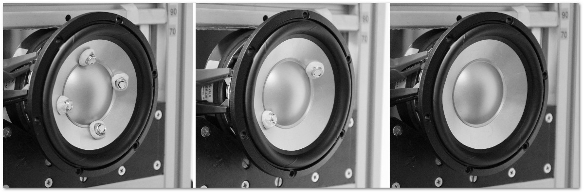
Measure the impedance with all 4 mass-loads ($m_2$, left panel) and save this data to the first ZMA file. Now very gently remove the two diagonal masses, leaving the remaining masses balanced and rocking modes prevented during the measurement of the speaker. Remeasure the impedance with the remaining two masses ($m_1$, middle panel) and save this data to a second ZMA file. Now very gently remove the two masses leaving the bare cone (right panel). Measure the impedance of the unweighted cone and save this data to a third ZMA file.

We use Blu Tack for added-masses, with a non-magnetic metal nut or coin optionally embedded for increased density. Be aware that magnetic materials can interact with the magnet system giving spurious results!

As the masses are removed from the cone, please measure their weight again and ensure that you know how much mass you've removed from the cone. These masses should be the values you measured before. The reason we measure in reverse order, as described above, is because applying the masses to the speaker may stress the mechanical suspension parts, which alters the viscoelastic properties. It is easier to remove the masses without stressing the parts and potentially without the cone moving at all. This will ensure the highest possible precision in determining all parameters, including the viscoelastic $\beta$ value.

Measurement equipment, which supports saving impedance measurements in the ZMA file format (that we're aware of):

• Smith & Larson Woofer Tester Pro (verified to work, highly recommended)
• ARTA LIMP (software only)
• Room EQ Wizard (REW), using Text Export (software only)
• Dayton Audio DATS V3

We recommend a stepped-sine signal measurement such that all frequency points are measured under steady-state conditions. It is our experience that a fast Chirp or Farina sweep will not result in acceptable precision. If your equipment only offers sweep options, we recommend a slow sweep to achieve reasonably high accuracy. Note: REW and DATS V3 both use a sweep.

Good luck.

We provide a web app to collect the previous impedance measurements (and masses) into a single file. This single (JSON) object can be stored on your computer locally and later uploaded into the parameter fitting app. In principle this step is only a required step because we felt is was a practical way to store measurements, a practical way to feed the data to the fitter, and should anything strange occur, a practical way for you to share the data with us so we can potentially investigate.

The data collection app requires the following input:

1. ZMA file containing impedance measurement of unweighted driver
2. ZMA file containing impedance measurement of driver with added mass $m_1$
3. ZMA file containing impedance measurement of driver with added mass $m_2$
4. The value of $m_1$ in grams
5. The value of $m_2$ in grams

This app also provides an optional comment field. We recommended that you type the driver name into this field. An optional field for specification of the input voltage is also available. Specifying the voltage is not a requirement either, but it's good practice to notice this because we know that the parameter values will depend on the input level. Remember to fill out these optional fields before you complete entering the five inputs.

The comment field is the first entry in the data object such that if you open up the file in a text editor, you can read your comment in plain text (at the top). This will help you identify the measurement. When measuring your driver, we recommend that you follow our measurement procedure.

For the three measurements in the ZMA files, all three measurements must contain the same data points (at the same measurement frequencies). It is not allowed to e.g. reduce the frequency range for some of the measurements.

This app uses the data stored in the previously generated JSON data container to generate a nonlinear fit to the advanced driver model. The free-air impedance in this model is given by

The equivalent electrical circuit for the driver in free air is

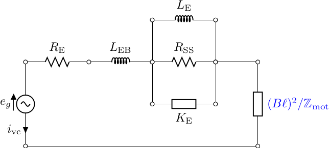
The parameter $\omega_0$ is set to $\omega_0 = 1.5 \cdot 2 \pi f_s$, where $f_s$ (the driver resonant frequency in Hz) will be determined by the fitting process. Some aspects of the dual-added-mass algorithm are described in our AES article, whereas other aspects are proprietary. The fit procedure is complicated, but provides a robust and accurate estimation of the model parameters. The advanced model utilizes what we consider to be the best analytic forms for both the electrical impedance (the Thorborg-Futtrup inductance model) and the mechanical impedance (the Knudsen-Jensen LOG model of viscoelasticity, with the added Retardation Spectra function as described by Agerkvist-Ritter). The fit parameters are suitable for high-accuracy loudspeaker box simulations (for designing loudspeaker systems). Please note that all information (including input variables and results) is stored in your browser and nothing is saved to the server (not even temporary data). At the end you should export the data and save the results to your local hard drive. If you don't and close the browser window, the data will be lost.

To compute the fit, simply upload the JSON container of the previous section into the app.

The fit analyzes your data and the fit result and provides you with a quality rating: Excellent, Good, Fair or Sorry.

We published an article in the "Loudspeaker Industry Sourcebook 2020" about Speakerbench, which explains some aspects of the fitting and how to analyze the results. Please see LIS 2020 pages 124-131 [2].

The Import tab ('page') in the Datasheet Creator application is a simple way to load one of a few predefined drivers into the creator. When working with your own measurements, please ignore this.

The datasheet creator takes input from the fitter. The purpose of the creator is to add information to your dataset such that it becomes enough information to constitute a complete datasheet for the driver (but without frequency response graphs or other pictures). This complete dataset may be filed on your computer locally and/or shared with others.

To be able to save the data, you must add the Brand and Model number

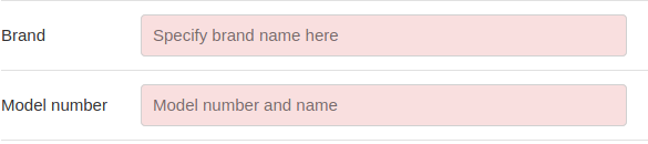
as well as the effective piston driver area (or diameter)

It is customary to add $X_{MAX}$, which is found available under the Simple tab, but it is not required by Speakerbench although some box simulation software might require this.

Once these additional parameters are added, the data object will be sufficient for box modeling. Beyond the necessary input data, you can provide additional information for the datasheet which may be useful in extreme environments; for example, air parameters (air temperature, barometric pressure, relative humidity) which are used for calculating $V_{AS}$.

Note: When you hover your mouse over a parameter, a tooltip appears and provides a brief explanation.

Here we offer a set of data, which you can use for testing the Speakerbench application, to see how it works, without having to measure your own data. We include data for all steps in the process. Just right-click on the links below and select "Save As" for downloading.

The point of measuring the driver and determining the parameters, is to be able to simulate (predict) the behavior in a box, before it is actually built. Here we offer a simple hands-on box simulation, with limited features, but we hope it is helpful as a first iteration (before exporting data to a proper box simulation software).

To load parameters for a driver into the box simulator, you need to use the Datasheet Creator app. When the data visible in the Datasheet Creator generates a JSON output, the data is stored in your local browser memory and 'automagically' shows up in the box simulator.

Hereafter you are able to insert box parameters in the 'Settings' tab and simulate the system behavior.

The box models supported by Speakerbench are:

1. Simple
   • The 'Simple' model just add a compliance, as specified by the box volume $V_b$. Damping material settings are ignored. All other features are supported. The model serves as a simple reference.
2. Futtrup
   • The 'Futtrup' model is a classic electrical equivalent circuit model, which adds the capability to simulate when damping material is added inside the box. It is an implementation of the 2011 AES paper by Futtrup.
3. T-net
   • The 'T-net' model treats the box using a transfer-matrix approach and describes the damping due to enclosure fill using Tarnow's equations (2002). We believe this is the most accurate approach.

All the enclosure models are accurate only for the low-frequency range, below the first box resonance.

With either the T-net or the Futtrup model you can choose between a number of different damping materials, either from Polyester or PET fiber, or from Glass wool (the number indicates the density in kg/m3).

For bass reflex simulation, Speakerbench supports two port models, one is classic (Simple), whereas the other includes port-resonances through a Transmission-line (T-line) model.

The Speakerbench box simulation supports simulation of the step-response, enabled by switching on the Time-domain (in the Settings tab). This is more calculation intensive, so we recommend to leave it off, until you wish to look at the 'Step' response graph. There are two plots, the time-pressure-response to an electrical step-input-signal on top, and below it the pole-zero plot. Since Speakerbench implements an advanced transducer model, with viscoelasticity and semi-inductance, the time domain response is calculated with a contour integral algorithm, as documented in our 2018 AES article.

At the bottom of the Settings tab, Speakerbench optionally supports the import of an impedance measurement as well as a frequency response measurement (can be Gain adjusted). This is helpful after having built the speaker and you wish to compare measurements with the simulation.

Alignment Chart

The Speakerbench box simulator provides an Alignment Chart, which might be helpful in selecting a suitable box volume and port tuning for your driver. The chart plots $\alpha = V_{AS}/V_B$ on the x-axis and $h = f_P/f_S$ on the y-axis. Within this chart, Speakerbench shows a blue cross with your current choice as well as some dots that represents well known alignments (known from Thiele/Small theory). These are:

Note: Only the alignments with limits that includes the $Q_T$ of the driver you have loaded will show in the chart. Unobtainable alignments are omitted.

With your mouse/pointer you may click anywhere inside the chart. Speakerbench registers the pixel where you clicked and the associated $\alpha$ and $h$ values, and when you go back to the Settings tab and push the APPLY button, the box volume and port tuning is updated accordingly.